Topic Distributions

BERTopic approaches topic modeling as a cluster task and attempts to cluster semantically similar documents to extract common topics. A disadvantage of using such a method is that each document is assigned to a single cluster and therefore also a single topic. In practice, documents may contain a mixture of topics. This can be accounted for by splitting up the documents into sentences and feeding those to BERTopic.

Another option is to use a cluster model that can perform soft clustering, like HDBSCAN. As BERTopic focuses on modularity, we may still want to model that mixture of topics even when we are using a hard-clustering model, like k-Means without the need to split up our documents. This is where .approximate_distribution comes in!

To perform this approximation, each document is split into tokens according to the provided tokenizer in the CountVectorizer. Then, a sliding window is applied on each document creating subsets of the document. For example, with a window size of 3 and stride of 1, the document:

Solving the right problem is difficult.

can be split up into solving the right, the right problem, right problem is, and problem is difficult. These are called token sets. For each of these token sets, we calculate their c-TF-IDF representation and find out how similar they are to the previously generated topics. Then, the similarities to the topics for each token set are summed to create a topic distribution for the entire document.

Although it is often said that documents can contain a mixture of topics, these are often modeled by assigning each word to a single topic. With this approach, we take into account that there may be multiple topics for a single word.

We can make this multiple-topic word assignment a bit more accurate by then splitting these token sets up into individual tokens and assigning the topic distributions for each token set to each individual token. That way, we can visualize the extent to which a certain word contributes to a document's topic distribution.

Example

To calculate our topic distributions, we first need to fit a basic topic model:

from bertopic import BERTopic
from sklearn.datasets import fetch_20newsgroups

docs = fetch_20newsgroups(subset='all',  remove=('headers', 'footers', 'quotes'))['data']
topic_model = BERTopic().fit(docs)

After doing so, we can approximate the topic distributions for your documents:

topic_distr, _ = topic_model.approximate_distribution(docs)

The resulting topic_distr is a n x m matrix where n are the topics and m the documents. We can then visualize the distribution of topics in a document:

topic_model.visualize_distribution(topic_distr[1])

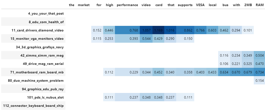
Although a topic distribution is nice, we may want to see how each token contributes to a specific topic. To do so, we need to first calculate topic distributions on a token level and then visualize the results:

# Calculate the topic distributions on a token-level
topic_distr, topic_token_distr = topic_model.approximate_distribution(docs, calculate_tokens=True)

# Visualize the token-level distributions
df = topic_model.visualize_approximate_distribution(docs[1], topic_token_distr[1])
df

Tip

You can also approximate the topic distributions for unseen documents. It will not be as accurate as .transform but it is quite fast and can serve you well in a production setting.

Note

To get the stylized dataframe for .visualize_approximate_distribution you will need to have Jinja installed. If you do not have this installed, an unstylized dataframe will be returned instead. You can install Jinja via pip install jinja2

Parameters

There are a few parameters that are of interest which will be discussed below.

batch_size

Creating token sets for each document can result in quite a large list of token sets. The similarity of these token sets with the topics can result a large matrix that might not fit into memory anymore. To circumvent this, we can process batches of documents instead to minimize the memory overload. The value for batch_size indicates the number of documents that will be processed at once:

topic_distr, _ = topic_model.approximate_distribution(docs, batch_size=500)

window

The number of tokens that are combined into token sets are defined by the window parameter. Seeing as we are performing a sliding window, we can change the size of the window. A larger window takes more tokens into account but setting it too large can result in considering too much information. Personally, I like to have this window between 4 and 8:

topic_distr, _ = topic_model.approximate_distribution(docs, window=4)

stride

The sliding window that is performed on a document shifts, as a default, 1 token to the right each time to create its token sets. As a result, especially with large windows, a single token gets judged several times. We can use the stride parameter to increase the number of tokens the window shifts to the right. By increasing this value, we are judging each token less frequently which often results in a much faster calculation. Combining this parameter with window is preferred. For example, if we have a very large dataset, we can set stride=4 and window=8 to judge token sets that contain 8 tokens but that are shifted with 4 steps each time. As a result, this increases the computational speed quite a bit:

topic_distr, _ = topic_model.approximate_distribution(docs, window=4)

use_embedding_model

As a default, we compare the c-TF-IDF calculations between the token sets and all topics. Due to its bag-of-word representation, this is quite fast. However, you might want to use the selected embedding_model instead to do this comparison. Do note that due to the many token sets, it is often computationally quite a bit slower:

topic_distr, _ = topic_model.approximate_distribution(docs, use_embedding_model=True)